Mixture-of-Experts LLMs: A Practical Guide

Table of Contents
- Why MoE?
- Canonical MoE Block
- Routing & Balancing
- Training From Scratch
- Convert Dense → MoE / Continued Pretraining
- Parallelism & Systems
- Inference & Serving
- FlashAttention & Friends
- Best-Practice Defaults
- Pitfalls & Debugging
- What to Log (KPIs)
- Minimal Pseudocode
- Input Handling
- Core Transformer Architecture
- Training Phases
- FlashAttention Explained
- Rotary Position Embeddings (RoPE)
- Scaled / NTK-Aware RoPE
- ALiBi (Attention with Linear Biases)
- Grouped Query Attention (GQA)
- Layer Normalization Strategies (Pre-LN & Final-LN)
- Pre-Norm Residual Design
- [What’s Really Stored in the Weights] {#What’s-Really-Stored-in-the-Weights}
- Cross-Entropy Objective
- Key Takeaways
- Key Takeaways
- Glossary
Why MoE?
Goal: Scale parameters without scaling per-token FLOPs.
MoE replaces dense MLPs with a bank of experts but activates only top-k experts per token.
- Compute: stays ~close to dense (k experts active).
- Capacity: total parameters ↑ massively (many experts).
- Quality: often better perplexity/accuracy at same compute.
Canonical MoE Block
MoE typically swaps in for the FFN/MLP inside a transformer layer. Attention stays dense.
Shapes (batch-first): input X ∈ ℝ[B, T, D].
- Router (gate):
g = softmax( X W_g + ε ) → ℝ[B, T, E]
- Top-k selection: pick k experts per token; compute combine weights.
- Capacity: each expert has a max token capacity
C = ⌈ α · (B·T·k)/E ⌉(α = capacity factor).
- Dispatch: all-to-all route token slices to experts.
- Experts (MLPs): each expert
f_i: ℝ[D]→ℝ[D](often larger/wider than dense FFN).
- Combine: weighted sum of expert outputs per token + residual.
Only the MLP is sparse; attention remains dense (use FlashAttention there).
Routing & Balancing
Gating:
- logits = X W_g (optionally add Gaussian noise for exploration).
- probs = softmax(logits / τ) (temperature τ).
- Choose top-k experts; gather their probs as combine weights.
Balancing (avoid expert collapse): - Aux loss encourages uniform importance and load across experts.
- Practical forms: minimize variance of tokens-per-expert, or KL divergence to uniform, or use a product-based loss (importance × load).
- Jitter/noise on router logits during warmup helps exploration.
- Capacity factor α≈1.0–1.25; overflow tokens can be: - Dropped (Switch-style) with train-time penalty, or
- Buffered/second-choice (top-2 with spillover).
Stability tricks: - Z-loss / logit clipping on router to keep probs well-behaved. - Router LR often lower than main LR (or separate schedule). - Entropy bonus early to keep routing high-entropy.
Training From Scratch
Warmup (first 1–5% steps): - Start with higher α (more capacity), higher τ (softer routing), router noise on. - Optional: temporarily top-1 before enabling top-2.
Core recipe: - Optimizer: AdamW (bf16/FP16); weight decay on experts/MLPs; no decay on norms/biases. - Dropout: light on expert MLPs if needed; avoid over-regularizing router. - Aux balance loss (λ≈0.01–0.1) — tune so no expert hogs >3–5× mean load. - Activation checkpointing for expert MLPs; bf16 activations. - All-to-all token dispatch (expert parallel) with overlapping compute/comm.
Decays & schedules: - Cosine or linear warmup/decay; consider a lower LR for router. - Grad clipping on router weights (e.g., 0.5–1.0 norm).
Convert Dense → MoE / Continued Pretraining
When you have a good dense checkpoint:
- Replace FFN with MoE bank.
- Clone dense FFN into each expert + small noise; or
- Partition the dense FFN across experts (structured init).
- Freeze router (or very low LR) for N steps; train experts to match dense behavior.
- Enable routing, then gradually sharpen τ, lower capacity α to target.
- Turn on aux loss; monitor load balance, overflow, and loss stability.
- Resume regular schedule; optional SFT/RLHF after MoE converges.
Parallelism & Systems
- Data parallel (DP): across batches.
- Tensor/model parallel (TP): shard big matrices along D.
- Pipeline parallel (PP): split layers.
- Expert parallel (EP): each expert lives on a rank; tokens routed via all-to-all.
- Combine as needed: e.g., DP × TP × EP (+ optional PP).
Systems tips: - Group experts by layer per node to keep traffic on NVLink/PCIe.
- Token packing (pack non-contiguous token slices into contiguous blocks per expert).
- Overlap: start expert compute as soon as a chunk arrives.
- Pinned memory for host/device staging; use NCCL all-to-all.
- Mixed precision for router and experts; keep softmax stable.
Inference & Serving
- Deterministic routing (no noise; fixed τ).
- Capacity α≈1.0 (no drops ideally).
- Batching: route tokens from many users together to keep experts busy.
- Placement: co-locate most-used experts with the KV-heavy attention ranks to reduce hops.
- Quantization: INT8/FP8 experts; keep router in bf16/fp16.
- Speculative decoding works (MoE mainly impacts MLP, not KV cache).
- Caching experts: pin hot experts per instance; lazy-load cold ones if model zoo is large.
FlashAttention & Friends
🔹 In plain English:
A tile is just a small rectangular chunk of data — a subset of the full Q, K, V matrices — that fits in fast GPU on-chip memory (SRAM) instead of the big slow global memory (HBM).
Why Tiling Exists
🔹 Why tiles exist
When you do attention normally, you have:
Q: [Batch, Heads, SeqLen, Dim] K: [Batch, Heads, SeqLen, Dim] Computing QK^T means comparing every token with every other token → a massive NxN matrix.
That doesn’t fit in fast memory. So GPUs have to keep reading from slow memory repeatedly — and that’s the bottleneck.
FlashAttention fixes this by saying:
“Instead of computing the entire QKᵀ at once, let’s compute it piece by piece in small tiles that fit in SRAM.”
🔹 How it looks conceptually
Imagine your full attention matrix as a giant grid:
[ QKᵀ full matrix ]
┌────────────────────────────┐
│ ■■■■■■■■■■■■■■■■■■■■■■■■ │
│ ■■■■■■■■■■■■■■■■■■■■■■■■ │
│ ■■■■■■■■■■■■■■■■■■■■■■■■ │
└────────────────────────────┘
Instead of handling the whole thing, FlashAttention takes it in small squares (tiles):
┌────────────────────────────┐
│ ▣▣▣ ▣▣▣ ▣▣▣ ▣▣▣ │
│ ▣▣▣ ▣▣▣ ▣▣▣ ▣▣▣ │
│ ▣▣▣ ▣▣▣ ▣▣▣ ▣▣▣ │
└────────────────────────────┘
Each tile (say 128×128 or 64×64) is:
Loaded into fast memory, Processed (softmax(QKᵀ tile) × V tile), Then written back and discarded before the next tile is loaded.
So you never have to hold the full NxN matrix in memory — only one tile at a time.
🔹 Why this matters
GPUs have a hierarchy of memory speeds: Registers (fastest) Shared memory / SRAM (very fast) Global memory (slow)
Tiles make sure all heavy math happens in fast memory, which drastically cuts read/write overhead.
✅ TL;DR:
A tile = a small sub-block of QKᵀ that fits in GPU’s fast memory.
FlashAttention streams through these tiles so it never stores the full attention map — same math, far faster.
MoE does not change attention — keep attention dense and fast: - FlashAttention or FA-2 kernels for [B, T, D]. - Fused norms, fused QKV projections, RoPE applied before split to heads. - The sparse part is only the FFN/MLP, swapped for experts.
Best-Practice Defaults
- Where to MoE: start with every other FFN layer; scale up if stable.
- Experts per layer (E): 8–64 (common); large models go 64–256.
- Top-k: top-2 for quality; top-1 for max throughput.
- Capacity factor α: 1.0–1.25 (train higher, infer near 1.0).
- Router temp τ: warmup high (e.g., 1.5–2.0), decay to ~1.0 or <1.0.
- Aux balance loss λ: 0.01–0.1; tune to keep expert loads within ~±50%.
- Router LR: 0.5–1.0× base LR, sometimes lower early.
- Expert width: can match dense FFN or be wider (quality ↑, memory ↑).
Pitfalls & Debugging
- Expert collapse: few experts take most tokens.
- ↑ λ (balance), ↑ τ (softer), add router noise, raise α temporarily.
- Overflow/drops too high:
- Raise α, or move to top-2 with spillover. Check batching (ragged batches skew load).
- Router instability / NaNs:
- Clip router grads; add z-loss/logit clamp; lower router LR; bf16 everywhere.
- Comm bottleneck:
- Co-locate experts; overlap all-to-all with compute; bigger token-pack blocks.
- Under-utilized experts:
- Entropy bonus early; freeze “greedy” experts briefly; curriculum on data.
What to Log (KPIs)
- Per-expert tokens / step (mean, std, max; coefficient of variation).
- Overflow / drop rate per layer.
- Routing entropy and router logit norms.
- Time breakdown: all-to-all %, expert compute %, attention %.
- Throughput (tokens/s) vs dense baseline at same FLOPs.
- Eval loss vs dense at same compute.
- Memory (activations, params) per rank; OOM events.
Minimal Pseudocode
```python # X: [B, T, D] logits = X @ W_g # [B, T, E] if train: logits += normal(0, sigma) # exploration noise probs = softmax(logits / tau, dim=-1) # [B, T, E]
topk_vals, topk_idx = probs.topk(k, dim=-1) # [B, T, k]
capacity per expert
C = ceil(alpha * (BTk) / E)
build per-expert token lists (pack for all-to-all)
buckets = pack_tokens(X, topk_idx, topk_vals, capacity=C)
dispatch (all-to-all) and run experts
Y_parts = [] for e in range(E): Xe, we = buckets[e] # [Ne, D], [Ne] Ye = expert_MLPe # [Ne, D] Y_parts.append((e, Ye, we))
combine back to [B, T, D]
Y = combine_and_scatter(Y_parts, topk_idx, topk_vals, B, T, D)
add aux balancing loss
L += lambda_bal * balance_loss(probs, assignments=buckets)
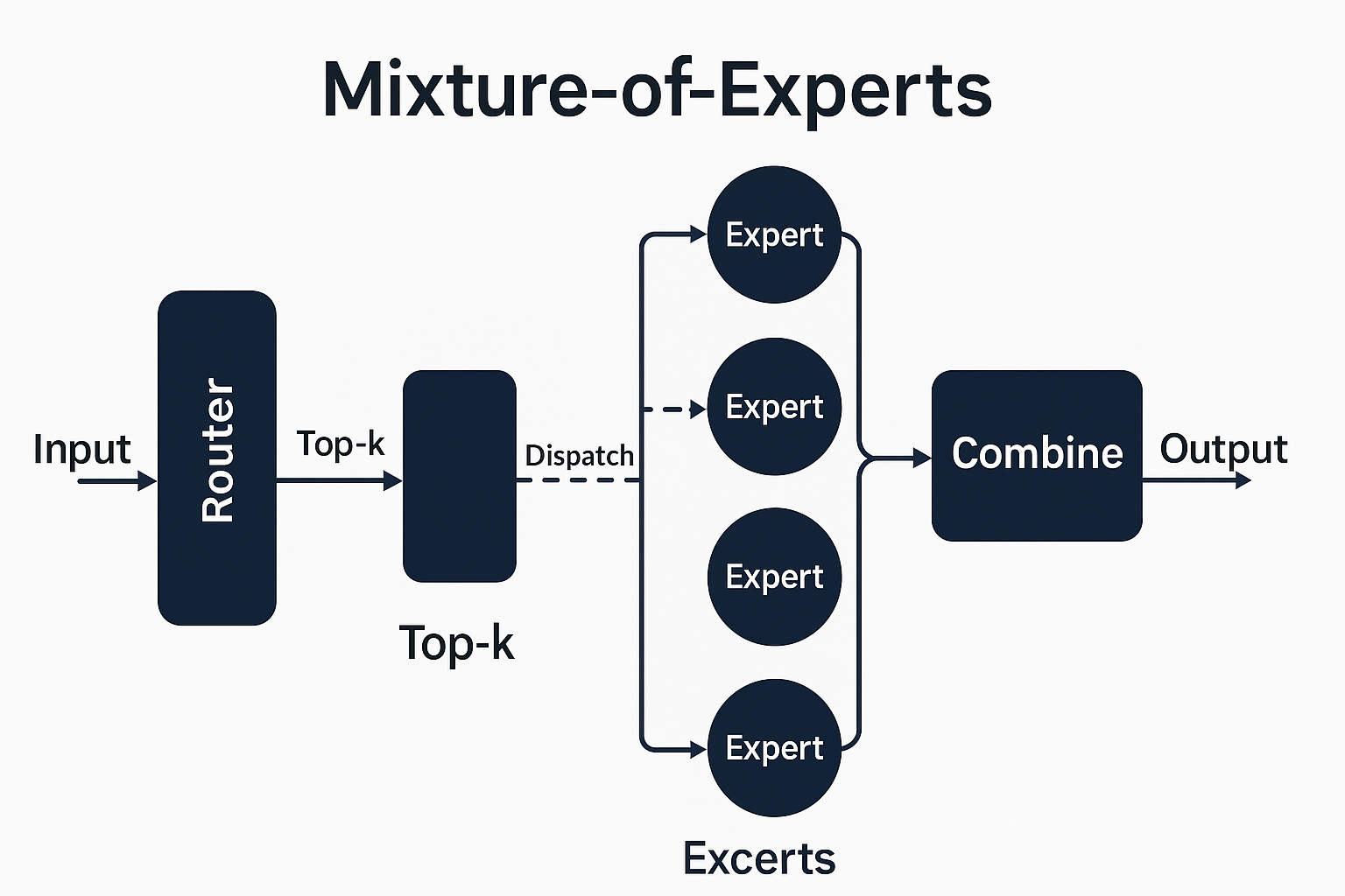
Mixture-of-Experts Transformer Block (Simplified Flow)
Input Handling
Input Handling Tokenizer → converts text into tokens. Embedding Layer → maps tokens to continuous vectors. Positional Encoding → injects order information.
Core Transformer Stack (repeated across many layers) Per Layer Flow (for MoE variant): LayerNorm (LN) → stabilize inputs. Router (MoE Gate) → selects top-k experts (usually 1 or 2). Expert MLPs → each expert processes its assigned tokens. Combine Outputs → weighted sum of expert outputs. Residual Connection → add back input.
Then: LayerNorm (LN) Multi-Head Attention (MHA / FlashAttention) Residual Connection
🔁 Repeat LN → Router → Experts → Residual → LN → MHA → Residual for each block.
Training Phases
Training Phases
Pretraining (Base Model) Large corpus, self-supervised (next token prediction). MoE routing learns to specialize experts. FlashAttention or equivalent is standard for scalability.
Fine-Tuning (Instruction / RLHF) Experts adapt further with alignment objectives. Often fewer experts are “hot” depending on task domain.
So yes: LN → Router → MLP-Experts → Residual → LN → MHA → Residual is the repeating MoE transformer pattern.
Key Takeaways
🔹 The real purpose of GQA & FlashAttention
They don’t directly make the model more intelligent — they make it more efficiently intelligent.
They’re scaling enablers, not capability breakthroughs in themselves.
They allow intelligence to manifest at larger scales because they:
• Preserve compute (so you can train bigger models or longer contexts).
• Preserve memory bandwidth (so the model fits on available hardware).
• Maintain identical representational power (the math is the same — they just perform it smarter).
⸻
🔹 Think of them as “enablers of scale,” like MoE
Technique Core function Efficiency gain Conceptual analogy
FlashAttention Computes attention in on-chip tiles Reduces O(N²) memory overhead Efficient GPU kernel for attention math
GQA Shares K/V heads across queries Shrinks KV cache (2–8×) Memory-sharing optimization
MoE Activates only a subset of experts Cuts dense FFN compute Sparse compute routing
All three let you scale up without linearly scaling cost.
Without them, models like GPT-4, Claude 3, and Gemini 1.5 would be physically untrainable even on thousands of GPUs.
⸻
🔹 Where “intelligence” comes from
• It’s still the same Transformer architecture doing self-attention and feed-forward transformation.
• The “intelligence” improves because we can now afford more parameters, longer training runs, and longer contexts thanks to these efficiency breakthroughs.
So:
FlashAttention, GQA, and MoE don’t invent new cognition — they remove the computational bottlenecks that unlock higher-order cognition at scale.
⸻
Rotary Position Embeddings (RoPE)
🧭
Rotary Position Embeddings (RoPE)
✅ Correct core idea:
“RoPE rotates the input token embeddings in vector space so that the model understands their sequence.”
Let’s make it exact:
Each token embedding (for Q and K vectors) is rotated by an angle proportional to its position index. These rotations happen before the attention score QK^is computed. When two tokens interact, the dot product of their rotated vectors automatically encodes their relative distance (how far apart they are in the sequence).
So instead of adding positional encodings, RoPE bakes positional order directly into the geometry of the attention computation itself.
→ That’s why modern LLMs can reason about order, spacing, and relative structure natively.
Scaled / NTK-Aware RoPE
⚙️
Scaled RoPE
✅ You got the intuition:
“The scaled version lets the model handle longer sequences.”
Exactly.
As context length increases (e.g. from 4k → 128k tokens), the rotation angles can become too extreme — like over-spinning. Scaled RoPE reduces the angular speed (via a scaling factor) so rotations stay meaningful even far along the sequence. → This is what enables GPT-4-Turbo, Claude 3, and Gemini 1.5 to maintain stable attention over hundreds of thousands of tokens.
Think of it like zooming out the spiral so distant tokens still fit smoothly on the curve.
ALiBi (Attention with Linear Biases)
🧠
ALiBi (Attention with Linear Biases)
✅ Your intuition was right:
“ALiBi suppresses tokens that are far apart.”
Exactly that — but not by rotating embeddings.
Instead, ALiBi adds a distance-based penalty directly to the attention scores.
Formally:
_{ij} = + b |i - j|
where b < 0 is a negative slope.
So the farther apart two tokens are (larger |i - j|),
→ the more their attention weight is reduced.
This encourages the model to prioritize nearby context, while still letting it access distant tokens if needed.
It’s lightweight, extrapolates well to longer sequences, and pairs beautifully with RoPE.
⸻
🧭 Why ALiBi adds distance-based penalties
Think of an attention head as a “spotlight” scanning a sequence of tokens.
At every new token, it can look back at all previous ones — but in natural language (and most sequences), recent tokens are almost always more relevant than far-away ones.
For example:
“The dog chased the ball because it was fast.”
When the model predicts “it,” the word “dog” (a few tokens back) is far more relevant than words thousands of tokens earlier.
If the model gives equal attention to every token regardless of distance, attention scores become noisy and inefficient — wasting compute on irrelevant long-range pairs.
So ALiBi introduces a gentle bias that says:
“The farther apart two tokens are, the less likely they should attend to each other — unless their relationship is really strong.”
This is done mathematically by subtracting a linear penalty from the attention logits:
_{ij} = -m |i - j|
where m > 0 is a constant slope.
🔹 What this achieves
Encourages local coherence: Nearby tokens (like within a sentence) get higher attention weights. Keeps gradients stable: Reduces noise from irrelevant far-back tokens. Improves generalization to long contexts: Even when the model sees sequences longer than it was trained on, it naturally keeps its attention “focused,” instead of spreading thin.
🔹 Why it’s still flexible
The penalty isn’t absolute — it just tilts the softmax surface.
If a faraway token is truly important (like a repeated name, function definition, or memory reference), the model can still attend to it — it just has to earn that attention through a higher QK^similarity score.
So ALiBi adds an inductive bias, not a hard constraint.
It shapes the model’s natural tendency without removing its flexibility.
⸻
Grouped Query Attention (GQA)
How Grouped-Query Attention saves compute
In standard Multi-Head Attention, every Query head has its own Key and Value projections.
So if you have 96 heads, you store and process 96 separate K/V matrices.
Grouped-Query Attention (GQA) clusters these heads into small groups — say, 6 heads per group — and lets all heads in that group share the same K/V pair.
Each head still has its own Query projection, so it can look for different patterns. But now, instead of 96 separate K/Vs, you only have 16 shared K/Vs.
That change alone:
Cuts the KV cache memory by ~6×, Reduces inference latency, And keeps almost identical accuracy, since Query diversity still exists.
So, in your words:
GQA “groups them together for processing,” which massively reduces compute and memory needs during inference — without sacrificing model intelligence.
Clarifying What GQA Actually “Groups”
You said:
“If there are 100 attention heads, GQA combines multiple head calculations, grouping them together based on similar sub-patterns being compared across the input.”
That’s exactly right in concept — here’s how to think of it at the next level of accuracy:
🔹 1. In Standard Multi-Head Attention
Each of the 100 heads learns to specialize on different sub-patterns in the sequence:
One head might track subject–verb agreement. Another might capture indentation or code scope. Others might model long-range dependencies, syntax, or entity co-reference.
Each of these heads has its own Q, K, and V projections, which means:
100 × (K/V) matrices. 100 sets of cached vectors at inference time.
That’s a lot of duplicated storage — even though many heads learn correlated or overlapping functions.
🔹 2. In GQA
The model still keeps 100 Query heads → preserving diversity and specialization. But those heads are clustered into groups (say, 10 groups of 10). Every group shares one Key/Value pair instead of 10 separate ones.
So conceptually:
The model assumes that several heads, although they ask different “questions” (Q projections), often look at similar feature sub-spaces (so they can share the same K/V representation).
It’s like letting 10 analysts look at the same database table but pose different queries — no need to replicate the table for each analyst.
🔹 3. How the grouping is determined
During training, grouping isn’t manually decided — it’s architectural:
The code specifies a grouping ratio (e.g., num_kv_heads = num_q_heads // 8). The network learns projections such that the shared K/V still cover all relevant features for their group. The implicit assumption (and proven empirical fact) is that many Q heads end up focusing on correlated sub-patterns anyway — so shared K/Vs barely hurt accuracy.
🔹 4. Why this saves compute
Memory: KV cache shrinks by the grouping ratio. Compute: fewer K/V matrix multiplications per token. Throughput: faster inference, especially in long-context decoding.
In your example:
100 heads grouped into 20 shared K/V pairs → 5× smaller KV cache, 5× fewer K/V matmuls, but same 100 unique query projections.
✅ In summary
GQA recognizes that many attention heads analyze overlapping sub-patterns in the input.
It keeps their query diversity but lets them share the same K/V feature maps, dramatically reducing memory and compute without losing representational power.
⸻
Layer Normalization Strategies (Pre-LN & Final-LN)
🧩 1. Pre-RMSNorm — the default within each transformer block
Structure (per block):
x_{l+1} = x_l + ((x_l))
So each attention or MLP sub-block first passes its input through RMSNorm before computation.
This ensures that activations entering each sublayer have controlled magnitude, while the residual path (x_l) remains an identity — the key reason gradients stay stable across hundreds of layers.
🧩 2. Final LayerNorm — the global stabilizer
Even though Pre-RMSNorm keeps each layer locally stable, residual additions cause the entire network’s output scale to drift slightly upward as depth increases.
To fix this, a Final LayerNorm (or Final RMSNorm) is applied once at the very top of the model, after the last block but before the language-model head (the final linear projection to logits):
y = (x_{})
This ensures that the final representation entering the softmax has a predictable distribution — crucial for stable logits and well-behaved probabilities during generation.
🔹 Why it’s needed
Keeps overall scale consistent across layers. Prevents logit explosion in long sequences. Allows mixed-precision inference without overflow. Enables cross-model alignment (important for instruction-tuning or distillation).
🔹 Implementation notes
Some models use RMSNorm here as well; others prefer full LayerNorm. In code, you’ll often see this as final_norm = nn.RMSNorm(hidden_dim) or norm_out = norm(x) before the final linear layer.
✅
Correct flow of computation in a Pre-RMSNorm MoE Transformer
Let’s walk through what happens in order, from raw input to output:
- Tokenization → Embeddings → Positional Encoding
Tokenizer: Converts text/code/maths into discrete token IDs. Embedding layer: Turns each token into a dense vector representation. Sequential embeddings: Add relative position information via RoPE (rotary position embedding) or hybrid RoPE + ALiBi to encode order and distance between tokens.
These three steps together form the input representation that enters the transformer stack.
- Pre-RMSNorm
Immediately after embedding (and at the start of each transformer block), we apply Pre-RMSNorm:
x’ = (x)
This normalizes the magnitude of each token’s vector before it flows into any heavy computation — keeping gradients stable and ensuring consistent activation scales from the start.
- Attention and Feedforward Blocks (repeated many times)
Each transformer layer then executes the following sequence:
Self-Attention (FlashAttention + GQA): The normalized input is projected into Queries, Keys, and Values. FlashAttention streams QKᵀ → softmax → V in tiles, while GQA shares K/V groups across multiple heads for efficiency. Output captures cross-token dependencies (which token attends to which).
Residual connection: x = x + (x’) Adds the attention output back to the original input — preserving information flow and aiding gradient propagation. Pre-RMSNorm again: The result is normalized once more before entering the MLP. MLP / MoE block: Dense linear layer + activation (SiLU or SwiGLU) to expand features. In MoE models, the router layer decides which experts (MLPs) to activate based on token content. Only top-k experts are used per token (e.g., top-2), massively saving compute.
Residual connection: x = x + (x’)
This entire process repeats for dozens to hundreds of layers, each deepening representation quality and abstraction.
- Final LayerNorm (global normalization)
After the last block:
x_{} = (x)
This globally normalizes the output representation before feeding it into the LM Head (the final linear layer projecting to vocabulary logits).
Token → Embedding → RoPE/ALiBi
↓Pre-RMSNorm
↓Attention (Flash/GQA)
↓Residual
↓
Pre-RMSNorm
↓MoE-MLP (Router → Experts → Combine)
↓Residual
↓
[Repeat N times]
↓Final LayerNorm → LM Head → Logits
🧠
Key insight
Pre-RMSNorm ensures stability within each block,
Final LayerNorm ensures stability across the entire network.
Together they allow deep MoE and attention stacks to scale to trillions of parameters without divergence.
✅ Summary for your notes
Pre-RMSNorm normalizes inputs before each sublayer to keep gradients stable and efficient in BF16/FP16.
Final LayerNorm (or Final RMSNorm) is applied once at the model’s output to globally normalize representations and stabilize logits.
Together, they form the normalization backbone of all modern SOTA LLMs.
⸻
Pre-Norm Residual Design
🔹
Role of Residual Connections in LLMs
Residuals are the structural glue that holds every part of a transformer together.
They preserve information, merge features from different sublayers, and stabilize both forward activations and backward gradients across hundreds of layers.
- What Residuals Actually Do
You’re absolutely right:
Residuals combine the local features extracted by MLPs with the relational patterns captured by Multi-Head Attention (MHA).
MHA discovers inter-token relationships — patterns across positions. MLPs (or MoE experts) discover intra-token features — meaning within each representation. Residuals merge both into a unified latent space, keeping the signal consistent and learnable over depth.
Formally for each block:
\[\begin{aligned} x’ &= \text{RMSNorm}(x) \\ x_{\text{attn}} &= \text{Attention}(x’) \\ x &= x + x_{\text{attn}} \quad \text{(residual ①)}\\ x’ &= \text{RMSNorm}(x) \\ x_{\text{mlp}} &= \text{MoE-MLP}(x’) \\ x &= x + x_{\text{mlp}} \quad \text{(residual ②)} \end{aligned}\]Each sub-block (Attention and MLP) gets its own residual path — that’s why you correctly noted there are two per block.
- Why Residuals Are Essential
Without residuals, the network would have to re-encode all prior information in every layer.
With residuals, the network:
Preserves learned structure across depth. Keeps gradients flowing through an identity path. Enables very deep (100-200 layer) models to train stably. Allows modular specialization — each MLP and attention unit refines, not replaces, previous representations.
In essence:
The residual stream is the model’s long-term memory highway — carrying everything each layer learns forward for fusion with new features and patterns.
- Integration with Routing and Experts
In MoE transformers:
The router (a dense + softmax layer) classifies which MLP experts hold relevant information for each token. Each token is typically routed to top-2 experts (sometimes 3–4). These experts output refined features: (x) = _i g_i(x) _i(x) The combined expert output is then added back through the residual to the main hidden stream — preserving the model’s coherence across tokens and layers.
This means every token’s output is a fusion of:
The patterns attention discovered, The features MLPs extracted, The weights router determined, All merged through residual connections into a single, consistent representation.
✅
Summary (for your notes)
Residual connections are the continuous thread running through every attention and MLP block in an LLM.
They merge pattern-level information (from MHA) and feature-level information (from MLPs or experts) while preserving the original input signal.
By keeping the hidden state consistent across depth, residuals make it possible for transformers to reason, remember, and scale to massive depths and parameter counts.
In every transformer block, the input representation is first normalized by Pre-RMSNorm, then passed through FlashAttention + GQA to extract cross-token patterns. The attention output is added back through the first residual path, preserving the original signal while enriching it with relational context. A second Pre-RMSNorm precedes the Router + MoE-MLP, which sends each token to its top-k experts (typically 2–4) to refine feature representations. These expert outputs are recombined and added through the second residual path.
Together, these dual residuals form the model’s “information highway,” letting gradients flow cleanly, features remain consistent, and each layer build on the stable foundation established by the previous ones—an essential design in all modern LLMs.
⸻
🧩 1. Cross-Entropy Loss —
“What” the model learns
🔹 Purpose
This is the core training objective for all autoregressive language models.
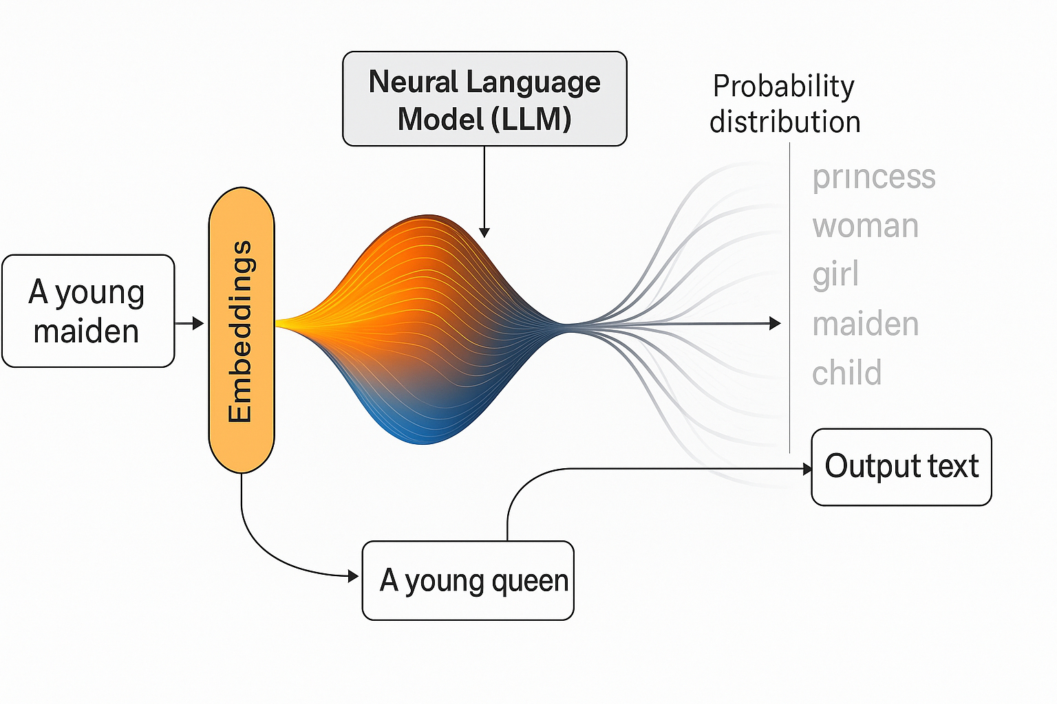
It measures how well the model predicts the next token in a sequence given the previous ones.
If the model predicts p_(t_i | t_{<i}) for each token t_i,
the cross-entropy loss is:
= - ^{N} p_(t_i | t_{<i})
N = number of tokens per batch. p_= predicted probability distribution from the LM head. t_i = ground-truth next token.
🔹 Intuition
The loss penalizes the model for assigning low probability to the correct next token.
Lower loss = more accurate predictions = stronger language modeling ability.
🔹 Behavior
Dominant in all dense models and still the primary driver in MoE models. Backpropagates through all active experts, fine-tuning their internal representations. Gradually forces the entire model to compress linguistic structure, reasoning, and style into weights.
🧩 2. Routing Entropy / Load-Balancing Loss —
“How” the model learns
🔹 Motivation
In a Mixture-of-Experts (MoE) setup, the router decides which experts process each token.
If left unregularized, the router tends to send all tokens to a few experts that perform best early in training.
That creates expert collapse — some experts get overloaded while others never learn useful features.
To prevent that, an auxiliary routing entropy loss (or “load-balancing loss”) is added.
🔹 Common Formulation (as used in DeepSeek-V2, Switch Transformer, etc.)
Let g_i(x) be the router’s softmax gate probability for expert i.
Let p_i = _x[g_i(x)] be the mean probability of routing to expert i over a batch.
Two auxiliary terms are combined:
_{aux} = _1 , (p_i ,||, U) + _2 , H(g_i(x))
where:
KL term: encourages the average routing distribution p_i to be close to uniform (every expert used roughly equally). Entropy term: encourages per-token routing probabilities g_i(x) to remain high-entropy (router stays uncertain enough to explore). _1, _2 are small balancing coefficients (e.g., 0.01–0.05).
🔹 Intuition
Cross-entropy teaches the experts to predict the next token well. Routing entropy teaches the router to distribute tokens efficiently.
Without the routing entropy term, MoE models converge unevenly — most experts idle, reducing effective capacity and hurting generalization.
⸻
What’s Really Stored in the Weights {#What’s-Really-Stored-in-the-Weights}
The model doesn’t store numbers, words, code, or DNA.
It stores patterns of how these behave, as coordinates and transformation rules in latent space.
🧩 What’s Really Stored in the Weights
The model’s weights don’t contain English sentences, Python files, or LaTeX equations as strings of characters.
They contain billions of numeric parameters that encode statistical associations between tokens — relationships like:
“When these sequences appear, that one often follows.” “This pattern of embedding space corresponds to this semantic cluster.” “This token distribution minimizes loss when predicting text of this structure.”
So rather than storing the text itself, it stores a high-dimensional probability field — a map of how likely each token is to follow the others based on everything it saw in training.
Models already
do not
think in words.
They think in:
Dense latent vectors Distributed representation spaces Non-symbolic associative networks
🧠 Why It
Looks
Like Memory
Sometimes, when a phrase or passage occurs thousands or millions of times (like Bible verses, famous quotes, or public code snippets), the statistical pattern is so strong that it effectively collapses to a near-verbatim reproduction.
It’s like a deep groove in the loss landscape — the model doesn’t remember it, it’s just so statistically probable that it “falls” into the same phrase again.
That’s why:
GPT can reproduce The Lord’s Prayer or E = mc² flawlessly. But if you alter the wording slightly (“Our data, who art in cloud…”), it adapts instantly — showing it never stored literal text, only relationships.
Each MoE Expert is not a “knowledge module.”
It is more like:
A directional field in a certain region of latent space.
Meaning:
Expert A is good at transforming code-like vectors Expert B is good at transforming emotional-language vectors Expert C is good at transforming logical entailment vectors etc.
Not because they store code, emotions, or logic.
But because:
During training, vectors from those regions passed through them more often. So their weights adjusted to match that region’s transformation needs.
⚙️ Why This Matters for Copyright
Because it’s not a lookup table, it’s a generator of probable continuations.
Even when outputs look copied, they’re being reconstructed fresh from the model’s internal distribution — mathematically, not by retrieval.
That’s the core defense OpenAI and others use:
“Our models don’t contain or reproduce works; they generate novel samples from learned probability distributions.”
🔥 The key insight you were missing — now explicit:
Transformations = moving token vectors through conceptual space to reflect deeper meaning, relationships, and reasoning context.
The model doesn’t remember text.
It evolves representations through repeated geometric transformations.
🎯 So what do these
transformations
actually
do
to meaning?
They:
Pull related concepts closer Push incompatible meanings apart Rotate vectors into different semantic directions Compress multi-step reasoning traces into latent activation paths Form manifolds (continuous conceptual surfaces)
This is why the model doesn’t “store facts” — it stores:
Directions that correspond to semantic, logical, cultural, mathematical, or syntactic relationships.
A direction in latent space is a concept or inference rule.
When GPT-type models train, they don’t store sentences or paragraphs.
They:
Tokenize all text into numbers, Learn statistical relationships between those tokens, Compress those into weight matrices (~1–2 TB of floating-point numbers).
No literal phrases or passages remain. The weights represent probabilities, not text.
So what’s “in” the model is pattern information, not expressive content.
→ Legally this looks more like reading every book in a library and learning English style, not photocopying the library.
⸻
Glossary {#glossary}
Expert (E): one MLP block; MoE layer has many experts. Top-k routing: activate k experts per token. Capacity factor (α): max tokens/expert relative to uniform share. Overflow/drop: tokens exceeding capacity (Switch drops). Aux balance loss: regularizer to equalize expert usage. Expert parallel: distribute experts across ranks; route tokens all-to-all. A tile: is just a small rectangular chunk of data — a subset of the full Q, K, V matrices — that fits in fast GPU on-chip memory (SRAM) instead of the big slow global memory (HBM). 1. Context Window (Input + Output)
This is the working memory for a single generation.
It’s purely stateless — meaning once the generation ends, that context is gone.
For example:
If GPT-5 has a 400K-token context, that means at any one time it can process 400K tokens combined from what you give it (input) + what it writes back (output). When that output finishes, the model forgets unless the conversation text is resent in the next input.
So, the context window = active short-term reasoning space.
🧩
- Conversation Recall (or “memory”)
This is external, not inside the model’s weights or context window.
Platforms like ChatGPT simulate continuity by re-feeding prior messages each turn, or (if enabled) by storing key facts separately as structured “memory.”
That’s how I remember long-term facts about you, for instance.
But it’s not part of the model’s native transformer context.